Use Python pandas NOW for your big datasets

Over the past few years I have been working on processing large analytical data sets requiring various manipulations to produce statistics for analysis and business improvement.

I quickly found that processing data of this size was slow, some taking over 11 hours to process which would only get worse as the data grew.

Most of the processing required multiple nested for loops and addition of columns to json formatted data, this had some large processing requirements and multi threaded processing wouldn’t help in these scenarios.

I knew there had to be a better way to process this data faster, and so I looked into using pandas.

What is pandas?

pandas is a software library written for the Python programming language for data manipulation and analysis. In particular, it offers data structures and operations for manipulating numerical tables and time series.

Test results

I ran some testing on 100 rows of data, one using for loops and one using pandas. With for loops the test took 19.09s to complete, with pandas an impressive 1.21s an improvement of 17.88s. When I run this on the full dataset which currently sits at around 16,500 rows it takes 33.15s seconds, an impressive improvement from a full run with for loops (which I had to cancel after 3 hours, it took too long for my requirements).

Pandas first steps

Install and import

Pandas is an easy package to install. Open up your terminal program (for Mac users) or command line (for PC users) and install it using either of the following commands:

poetry install pandas

OR

pip install pandas

Alternatively, if you’re currently viewing this article in a Jupyter notebook you can run this cell:

!pip install pandas

The ! at the beginning runs cells as if they were in a terminal.

To import pandas we usually import it with a shorter name since it’s used so much:

import pandas as pd

Series and DataFrame

The two main components of pandas are Series and DataFrame.

A Series is a column and a DataFrame is a table made up of a collection of Series.

DataFrames and Series are quite similar in that most operations that you can do with one you can do with the other.

Creating a DataFrame

DataFrames can be created multiple ways, I use PostgreSQL and BigQuery, using the pandas read_sql and read_gbq the data is automatically placed into a DataFrame.

Also we can manually create a DataFrame, using Python dict and list which is great for testing.

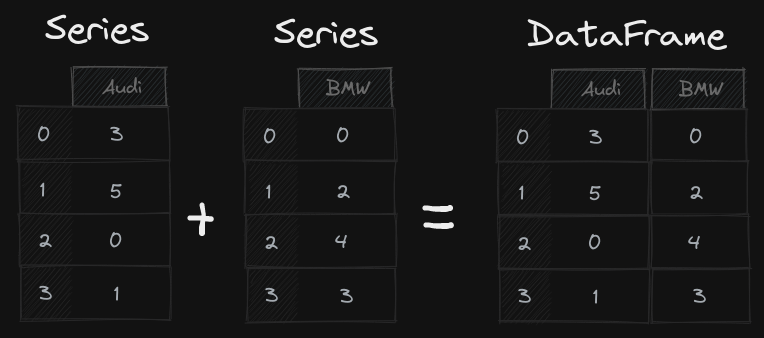
Taking our example in the diagram above, we have how many cars have sold each day. To organize this as a dictionary for pandas we could do something like:

sales_data = {
  'Audi': [3,5,0,1],
  'BMW': [0,2,4,3]
}
sales = pd.DataFrame(sales_data)

We would then see the data in the DataFrame format below:

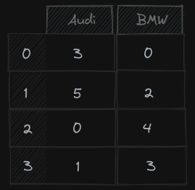
As you can see, each key from the dictionary is converted to a column, and the values are all put into a new row on the corresponding column

The Index of this DataFrame is given on creation, as numbers 0-3, but we could also create our own when we initialize the DataFrame.

sales = pd.DataFrame(data, index=['Jan', 'Feb', 'Mar', 'Apr'])

Iterating data

Normally with Python you would create iterate through data using a for loop to check every column, to do this with a DataFrame it would looks like this:

for sale in sales.itterrows():
  if sale['Audi'] > 5:
    print(f"Audi Targets hit with {sale['Audi']} sales.")
  if sale['BMW'] > 3:
    print(f"BMW Targets hit with {sale['BMW']} sales.")

This way of iterating through data is slow, I found this when I needed to do multiple nested for loops over multiple DataFrames.

However, there is a much faster and more efficient way to do this using the pandas loc function. So now we could locate a specific month’s order by using the month name:

sales.loc['Feb']

Audi  3
BMW   0
Name: Jan, dtype: int64

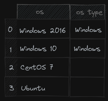
This example is quite simple, but we can get more complex with different data, for example if you had a list of servers with their operating systems you could find all server OS’s with “Windows” in the name and create a new column “OS Type” with “Windows” as the value to quickly filter by all Windows devices.

servers.loc[~servers['os'].isna() & servers['os'].contains("Windows").lower(), "OS Type"] = "Windows"

• servers - is our DataFrame
• .loc[] - Allows access to a group of rows and columns by labels or boolean array
• ~servers['os'].isna() - checks that the os column has a value
• servers['os'].contains("Windows").lower() - Checks that the os column has windows in the name and converts it to lower case to ensure all matches are not case sensitive.
• OS Type is the column to update if the statements match
• = "Windows" is the value to update the column with

Below would be the expected output from this Dataframe manipulation.

Merging DadaFrames

Much like doing a join with a SQL table, you can merge DataFrames based on specific columns:

pd.merge(
        devices,
        os_data[
            [
                "device_name",
                "operating_system"
            ]
        ],
        on=["device_name"],
        how="left",
    )

Final Thoughts

There is much more that can be done with pandas and DataFrames, this just scratches the surface and gives a very basic overview. The main reason for writing this article is to show what a difference in performance is made from using pandas, if you aren’t using this for your data yet, I recommend that you do!